Support Vector Machines
Overview
A Support Vector Machine (SVM) is a supervised machine learning algorithm designed for use in classifying data points. An SVM takes a collection of labeled training examples with various classes, looks for where the different classes are located, and seeks to find the best decision boundaries that separate observations from the various classes. The classic issue that arises from work of this type is that one is forced to decide between having too much bias or having too much variance. Low variance but too much bias implies that the found-boundaries between the classes are too simplistic. This often produces stable models, but they may systematically misclassify observation because the boundaries are too simple. Low bias but too much variance solves that problem, but now implies that the found-boundaries are overfitted for the data and will not necessarily classify new incoming test data correctly. SVM is a once-upon-a-time solution to how to best balance between these two worlds.
SVM does not attempt to simply separate the data correctly, but rather looks for the linear separator that leaves the largest possible margin between the classes, while allowing, when appropriate, a small number of observations to lie on the wrong side of the boundary. This much more nuanced approach accounts for the data to have a great variety of possible shapes of how the different classes might be geometrically oriented with respect to one another. The data might even be quite mixed together! SVM is a brilliant development that allows one to transform the data into a much higher-dimensional space and only then find a linear hyper-plane separating the categories. This novel approach developed in the 1990s was the industry leading technique for supervised classification for multiple decades.
To best explain Support Vector Machines, perhaps it would be wise to give a demonstration. Let's gather all the stats info on NFL running backs in the year 2000 and keep, specifically, the info on their rushing yards and their number of fumbles. Suppose one then gathers the info on which of those players retired at the end of the year and which players, instead, played on into the 2001 season. Here is a graph presenting that info:
Demonstration

Let's pair down this dataset to a much smaller number of players to better give a demonstration of how the machinery of SVM works.

(Note that a small number of quarterbacks and other positions are included in the rushing data. While they were not running backs, by position, in very early years of the NFL statistics, players were not always listed with their position. Some players were only listed with their number of yards, in mixed lists including quarterbacks, running backs, and wide receivers. For thoroughness, all players who ran the ball are included in the running data cube.)
Graphing the above dataset looks like this:
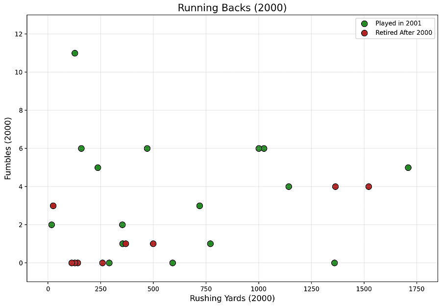
Linear Separation
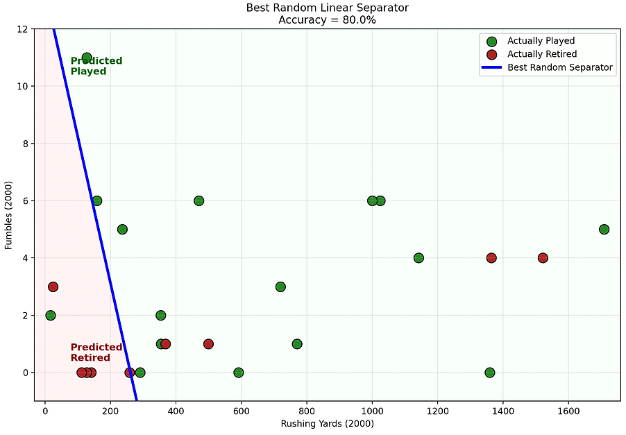
A classical, basic machine learning technique useful for this would be to find a line that best divides the data. Let's find just such a line and see how effective a classification tool it is. Brute force analysis will try many many lines and see which performs the best. Such a search is called a Monte Carlo search.
After trying 50000 random lines across the data, this one was the one found to be the best linear separator for the data, with an accuracy of 80%:
Support Vector Machines
Although the previous linear classifier performed reasonably well, the whole technique is fundamentally limited to separating the data with a single straight line. Support Vector Machines approach the problem differently. SVMs use a method of elevating the data up into a higher-dimensional space (using a feature-mapping function) and then finding a linear separator that well-divides the data. While 2D data can be separated using a line, high-dimensional data is divided using an analogous linear hyperplane. The data is then transformed back down into the original number of dimensions and leaves behind a separating decision boundary that is often quite curved.
SVMs provide an additional advantage over the traditional line separation method. Instead of merely trying to find a good line that divides the data, the SVM approach seeks the best linear separator that leaves the largest possible margin between the two classes. The observations lying closest to this boundary are called "support vectors" and determine the position of the higher-dimensional hyperplane. This lets SVMs be much more readily able to handle the complexities of real-world data which may have numerous small outliers present across the dividing line. Maxizing this margin between the classes is a more nuanced approach and generally produces classifiers that are less sensitive to small perturbations or isolated outliers and often generalize more successfully to previously unseen test data.
Constructing these higher-dimensional coordinates explicitly would quickly become computationally impractical as the number of features grows. What makes SVMs so clever is their use of "the kernal trick" which bypasses ever actually constructing the transformed, high-dimensional vectors. Instead the dot products of those vectors can be calculator directly as though one were performing the math on the high-dimensional vectors. This elegant mathematical shortcut makes it possible to obtain the benefits of high-dimensional classification, while preserving the runtime and low complexity of working with the original dataset.
To demonstrate how this process works, this project will next examine the two most common kernel functions: the polynomial kernel and the radial basis function (RBF) kernel.
Polynomial Kernel
The polynomial kernel is one of the simplest and most intuitive examples of the kernel trick. For this demonstration, the following degree-two polynomial kernel will be used:

This particular polynomial kernel has degree d=2 and constant offset of r=1 and is good for demonstration purposes due to its simplicity.
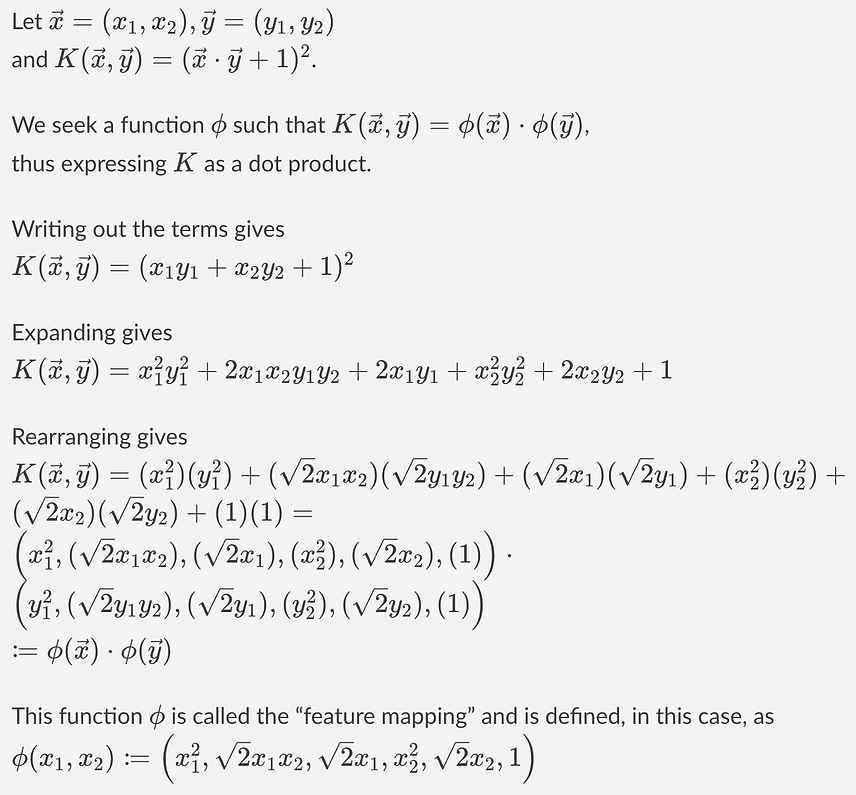
Let's demonstrate this transformation on two NFL players: P1 = Edgerrin James (1709 rushing yards with 5 fumbles) and P21 = Ricky Williams (1000 rushing yards with 6 fumbles).
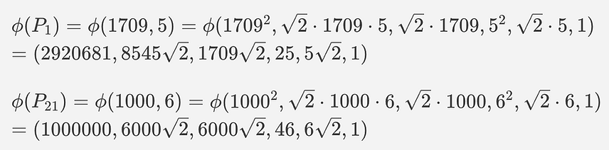
Once all the data is converted into its new 6-dimensional form, the next step is to search for the optimal linear separator hyperplane which creates the largest possible margin between the two classes within the data. While the earlier Monte Carlo search for the best line tried to find the best values of m and b in the equation y = mx + b, generating various separation lines, here the search for the best hyperplane involves optimizing w and b in the equation w • Φ(x) + b = 0, generating various hyperplanes. The optimization problem to be solved is:
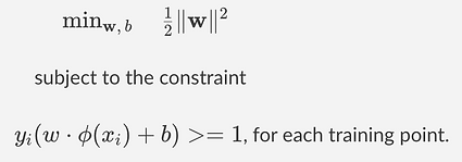
When one actually does the full optimization problem, using Lagrange Multipliers, one finds that the optimal value for w is
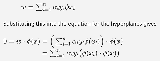
This final formula reveals what would be the runtime bottleneck. Finding the optimal hyperplane would involve performing many many calculations of Φ • Φ dot products. This is not so bad when the degree of the polynomial kernel is only d=2, creating vectors of only 6 dimensions, but in real-world machine learning use, the vectors end up being significantly high-dimensional. Calculating each of these, across all pairs of data points, in possibly very large data sets, would make the runtimes explode.
But this is the genius of the kernel function. It lets the machine learning algorithm bypass actually constructing the higher-dimensional vectors Φ(x) and Φ(y) all together! Recall that

This lets the machinary compute all the solutions for the higher-dimensional scenario using only the dot product of the original small, simple vectors! With this amazing breakthrough, SVMs with polynomial kernel become a very effective, practical solution to the problem of classifying data. Below are a few of the printouts for the NFL demo data with various polynomial kernels used for classification:
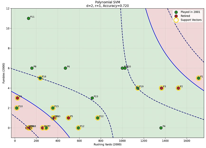


And after only trying a few polynomial kernels, already one has been found that beats the original linear divide's accuracy of 80% with a new best of 84%. With more complex data than this simplified little demo dataset, SVM reveals itself to be a truly powerful tool.
Radial Kernel
The polynomial kernel demonstrated a remarkable idea. Even though the original little demo dataset only had 2 dimensions, the kernel function behaved exactly as though every player had first been lifted into a higher-dimensional feature space before the SVM searched for the optimal separating hyperplane. For the example quadratic polynomial demonstrated above, the feature space contained six dimensions. The Radial Basis Function (RBF) kernel takes this idea and pushes it much further to even deeper abstraction.
The RBF kernel behaves as though ever observation has been tranformed into an infinite-dimensional feature space! Without the kernel trick, this would be impossible. But since SVM never actually explicitly constructs the infinite-dimensional feature vectors, it is able to perform the mathematics on them anyway using the shortcut. It evaluates a remarkably simple kernel function whose output is mathematically identical to the dot product that would have been obtained in that infinite-dimensional space.
The result is an algorithm capable of producing extraordinarily flexible decision boundaries while performing only straightforward computations on the original 2D dataset. Within the RBF system, nearby points strongly influence one another while further away points have rapidly diminishing influence.
The RBF kernel has this equation:
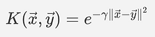
Unlike the polynomial kernel, this kernel depends on the distance between the two vectors, not on their dot product. Let's give an example using the same two players above: Edgerrin James, P1, and Ricky Williams, P21.
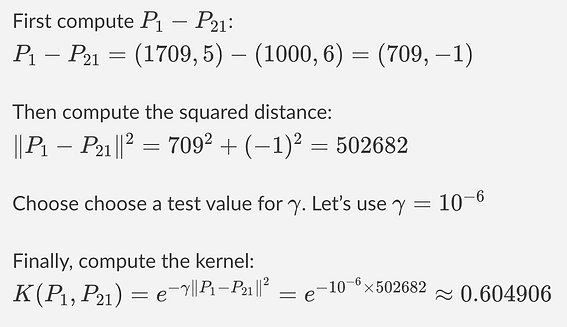
The RBF kernel always satisfies 0 < K(x,y) ≤ 1. Values near 1 imply the observations x and y are near to one another. Values near 0 imply the observations are very far apart. Due to the negative exponential nature of the radial kernel, when two observations are only of a medium distance from one another, the effect they have on one another diminishes precipitously. The rapidity of this is determined by the choice of value for gamma. Often when using radial kernel for SVM in machine learning, a variety of gamma values are tested for optimal classification.
Using radial kernel on the NFL demo dataset, provided with a few various values of gamma, produces the following classifications and associated accuracies:

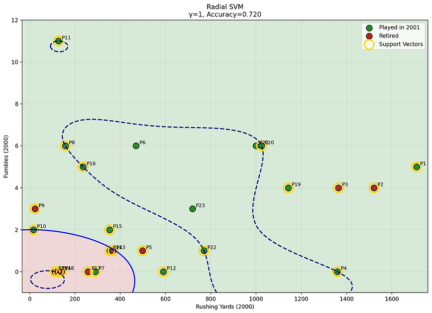

In almost no time at all, the radial kernel version of Support Vector Machines was able to classify the data the best that has been so far, achieving an accuracy of 96%. Support Vector Machines are a powerful tool and are capable of constructing highly flexible nonlinear decision boundaries.
Implementing SVMs into the NFL Predictive Machine
The core problem that makes it tricky to weave SVMs into the predictive machinary of the project is that SVMs are, at their core, a supervised categorizing algorithm, whereas my project involves numerical assessments of predicting the future of particular vectors. There is no immediately intuitive way to use SVMs to assist in the NFL predictions. That being said, where there is a will, there is a way. A little creativity was required.
The project will integrate support vector machines into the predictive machinery in the following manner: Suppose one begins with a specific historical player, Bob, and a given number of test years of Bob's career. Call that number of test years Z. The first question is did Bob play in year Z+1 or did Bob retire immediately after year Z. First the machine will gather all players of a similar position to Bob and prune from the data all of those who played for less than Z seasons. Then those will be classified into two groups. Those who retired after their Zth season and those who played on. Now the SVM algorithms can be run to separate those two groups with an appropriate decision hyperplane, and Bob can be classified as most likely belonging to one of those two groups. If Bob is predicted to immediately retire, then the algorithm concludes. If not, the data is once again pruned to have only players who at least played Z+1 seasons. These are then examined for their percentile scores in that Z+1th season. While all of the above SVM discussion only ever covered support vector machines dividing data into two groups (green and red), they actually excel at dividing data into multiple groups! Thus SVM can be used to divide those players into regions wherein the players's Z+1th season had a percentile score that falls into various bins, let's say 1.0 to 0.8, 0.8 to 0.6, 0.6 to 0.4, etc. Bob can then be classified into which of those bins he best fits into. Suppose Bob fits into the 0.6 to 0.4 bin. He will be assigned a prediction of the mean of that bin, aka 0.5. The algorithm then repeats for the Z+2th season, the Z+3th season, etc until the algorithm predicts that he will retire.
In this fairly unorthodox fashion, support vector machines will be able to be used to produce a numerical prediction set for the future of a given test player's NFL career.
Data Prep
There was an important decision to be made at this point. All of the above discussion leads to an algorithm that will be able to produce a prediction for the future of a player's career percentiles, but there is a problem. All of the stats on the known part of the test player's career are used to generate a percentile for how well they played in year Z+1, but only a percentile. Full stats for that next year are not generated. This means the same mechanism cannot then be recursively studied to make a prediction for year Z+2. This is very real problem.
One possible future path would be to have the SVM system additionally produce sythesized values for all of that player's future stats in each category, using the binning system at each step. This would dramatically reduce runtime efficiency and would begin to feel less scientific. More and more of the actual predictive machinery of the algorithm would be, for instance, producing its predictions for year Z+5 based on examining many years of full statistical data... that it just invented! This felt both less effective and less valid.
The other, perhaps also not perfect, technique was to have the entire SVM version of the predictive engine examine only players's career percentile scores. This means no longer would there be a distinction between rushing QBs and pocket passers. Kickers who excell at making 60+ yard kicks, but are a little less accurate making extra points. All that the algorithm would be seeing is simply how well a player played across their seasons. This was the direction that was chosen, for a mixture of maintaining a reasonable runtime and also in pursuit of research authenticity.
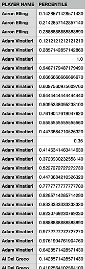
A new very simple code was composed designed to take the full data cubes and strip them of all their bells and whistles until only the player name and percentile score columns remain:
Before

After
Code
All of the code used in this portion of the project can be found via the following link. Each small specific experiment run will have a provided link to its own small sub-folder. But here is the link to the larger outer folder that contain all the code:
Testing for Optimal Parameters
Early version of the SVM-implementation of the NFL predictive engine had a problem with erring on the side of failing to spot when a player should appropriately retire. Almost all the predictions gave almost all the players future careers of maybe 10 or 13 more years. The issue was that at any given predictive future season, call it year Z+i, most of the players who've played Z+i-1 years do not retire precisely at their Z+ith year. This means that the SVM-based classifying was always dominated by those players who did not retire each given year.
A solution was found by implementing the following change. SVM has the capability of having any of the various decision bins be assigned a weight, thus making the algorithm more likely to classify test nodes into that category. It effectly nudges the largest-margin separator in the desired direction by making violations on that side more "expensive". Multiple values for the retirement weight were tested fairly extensively, and the optimal value proved to be approximately r=4 or thereabouts. This gave much more accurate predictions for player retirment.
Other variables had yet to be tested. Most notably, there was the issue of how many bins should player percentiles be separated into. The original explanation above discussed having five bins, roughly corresponding to letter grades. A player pecentile from 1.0 to 0.8 could be called an "A". One from 0.8 to 0.6, a "B". 0.6 to 0.4 a "C", etc. But there is no inherent reason why five bins is necessarily the best number of divisions. Extensive testing was performed for each of three various kernels — polynomial (with degree 3), radial, and an additional not discussed above called linear kernel. Linear kernel is another fairly common SVM kernel with the very-simplistic formula K(x,y) := x • y . Each was tested for the best number of bins, with the following results:
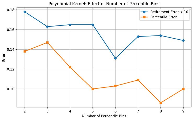


Radial and linear had a clear winner with b = 6 being the best value. Polynomial kernel was a little more nuanced with b = 6 being the best for retirement error, but b = 8 being the best for predictive error. The project chose to pursue the one that gave the minimal predictive error, as that is, ultimately the more interesting and complex of the two portions of the project.
For polynomial kernel, then there was the issue of how many degrees the kernel transformation function should be run with. An experiment was designed to test this, but it had the somewhat unexpected result of finding that polynomial kernel runs very slowly with higher kernels. After a full day of running the code, only the following graph was obtainable:
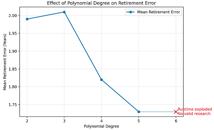
It's possible that higher-degree polynomial kernels might produce better, perhaps even quite-impressive results (!), but with the finite time within the constraints of the project, degree 4 was selected due to its quite-good predictions along with reasonable runtime.
Results
With all parameter values chosen, the predictive engine was finally ready for its ultimate evaluation. Each kernel was run against the same randomly generated collection of NFL careers, allowing for a fair, head-to-head comparison. The results below show how each different kind of SVM kernel performed:
Linear Kernel

Polynomial Kernel

Radial Kernel

The results were quite surprising! Both the polynomial and radial kernels surpassed the previous best mean retirement error (1.8315) achieved by the earlier K-nearest-neighbors version, and all three kernels produced lower mean percentile errors that the previous versions. This was very encouraging! Considering that support vector machines are traditionally used only for classification tasks, it was especially exciting to see that they could instead be used in an unorthodox manner to recursively classify vectors into various bins and produce a numerical prediction instead. Not only did this unconventional approach succeed, but it outperformed the project's earlier K-nearest-neighbors model on both evaluation metrics!
This work opens the door to additional testing and refining. Perhaps with further testing even more accurate version of the machine could be piloted. There is great interest in studying further testing and evaluation of slight adjustments of the various coefficients used in the making of the radial kernel in particular, the retirement weight value, the # of bins, etc. Another promising direction is to combine the recursive SVM framework developed in this project with the DecisionTrees, allowing multiple machine learning techniques to cooperate during the prediction process.
Conclusions
Perhaps the most significant lesson learned throughout this SVMs section of the project was that machine learning algorithms can sometimes be adapted to solve problems far beyond the tasks for which they were originally designed for. Support vector machines are traditionally viewed as classification algorithms, yet by combining repeated classifications with recursion and binning, they were transformed, with great success (!), into a machine capable of producing numerical forecasts for the remainder of an NFL player's career. This demonstrated that even algorithms with seemingly rigid purposes can become surprisingly flexible when incorporated into a larger predictive framework.
The experimental results were highly encouraging. Both the polynomial and radial basis function kernels surpassed the best mean retirement error previously achieved by the K-nearest-neighbors prediction engine, while all three kernels produced lower mean percentile prediction errors than the earlier approach. These results suggest that recursive machine learning techniques are capable of capturing long-term patterns in player development that simpler instance-based methods may fail to recognize. It was particularly exciting to discover that this unconventional adaptation of support vector machines not only functioned successfully but ultimately exceeded the predictive performance of the project's previous state-of-the-art model.
The project also reinforced an important principle of practical machine learning: predictive accuracy is only one component of a successful model. During experimentation, higher-degree polynomial kernels often produced improved predictions but at the cost of dramatically increased computation time. There is a real-world trade off, it seems, between perfecting the predictive engine and having it generate its predictions in a timely useful manner.
Finally, this work suggests several promising directions for future research. While only support vector machines were investigated here, the recursive prediction framework developed during this project is largely independent of the underlying machine learning algorithm. Decision trees, random forests, gradient boosting methods, neural networks, or even hybrid combinations of multiple algorithms could potentially be incorporated into the same recursive architecture. Exploring these possibilities represents a natural next step and may ultimately lead to even more accurate systems for predicting the future careers of professional athletes.