Principal Component Analyiss
Overview
Principal Component Analysis (PCA) is a widely-used dimensionality reduction technique used to simplify complex datasets while preserving as much of the information as possible. Often has the useful side effect of removing external noise from the data while keeping the core skeletal structure of the data intact.
As the number of dimensions of a data set increases beyond 2 or 3, visualizations become more and more difficult, computations become more runtime costly, and dramatic meaningful patterns may be completely obscured by noise. This phenomenon is often referred to as "the curse of dimensionality".
The goal of PCA is to transform a dataset into a new coordinate system whose perpendicular axes capture the greatest sources of variation present in the data. These new axes are called the "principal components". These often retain most of the information contained in the original data set. A scree plot can be used to offer a graphical representation of how much of the original variance in the data is captured by each of these new principal component directions.
PCA operates within the framework of Linear Algebra and is designed for use upon an m-by-n matrix of numerical data. This makes it perfect for use upon this project's NFL statistics data and requires no additional conversions or categorical hot encoding. Two key concepts within PCA are those of the eigenvalues and the eigenvectors. An eigenvector represents a direction in the data along which variation occurs, while the associated eigenvalues measure how much variation exists in that direction. Principal components are formed from the eigenvectors of the covariance matrix, and the components with the largest eigenvalues explain the largest amount of variation within the dataset. By pruning the data down to just those few eigenvectors associated with the largest eigenvalues, it is possible to reduce the dimensionality of the data while preserving as much of its structure as possible. Hence the name, Principal Component Analysis. PCA can simplify analysis, reduce noise, improve or make possible visualizations, and improve the performance of machine learning algorithms.
Two small visual examples of this process in action are offered here:


This project will apply the PCA technique to take the original large matrices of NFL data found in each of the five data cubes, transform the matrices into new dramatically simplified form, thus reducing noise in the data, and provide a scree plot for each type of NFL player being studied to see what are the most important principal components.
At that point, the career predictive method that currently has the "high score" will be reapplied to the data to see if the predictions thus generated are an improvement upon the original model.
Data Prep
If anything was learned in the previous section on clustering, it is that so far all of these machine learning tools have required the data cube to actually be "cube shaped", aka all of the dimensions need to be the same length, width, breadth, etc across the entire structure. The core problem that the K-Mean and especially the Hierarchical Clustering encountered was that NFL players have quite a great deal of variety in terms of how long they played for in the NFL. This means that one of the dimension of the cube is a jagged, variable, unpredictable-lengthed side. A quick mental image of that might appear something like:


Last time, with clustering, the predictive machine was instructed to simply pad the missing data all with -1's. This backfired spectacularly. It's possible that trying to pad the data with any sort of number is just fundamentally not going to work. This time the project will try something different and perhaps more original.
Suppose one is to compare two players, one of whom played for three seasons and one of whom played for ten. One could represent those vectors as [A,B,C] and [1, 2, 3, 4, 5, 6, 7, 8, 9, 10]. The core question is how can one get those two vectors to become of equal length. This time, the new concept is to 'stretch' out the first player's career, by repeating elements within the vector, until they are all of equal length. The first player's vector would now become [A, A, A, A, B, B, B, C, C, C] so that they are both of length 10. In the actual project, to keep things standardized and to make sure that even the players with the longest careers have their stats stretched as well, all the careers will be stretched out to 100 years each. To make sure that player's career still gets factored into how the machine is viewing and comparing their careers, an additional new column will be added that stores the length of each player's career. To make sure that this number is given appropriate weight, it will not be simply added to the data cube, but will be offered in x5 form, giving it additional oomph.
Here is a pre-transformation glimpse at the Runningback data cube:

The careers were all stretched to 100 years. An additional column was added to the right side of the column that stores the player's original career length x5. Here's a glimpse of the new transformed data:
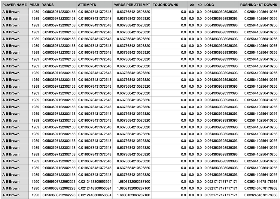
Lastly, one more bit of data transformation was needed to be able to perform PCA. All those many many duplicate rows all needed to get stacked beside one another instead of one top of one another. This resulted in five final PCA-ready data cubes.

Code
All of the code used in this portion of the project can be found via the following link. Each small specific experiment run will have a provided link to its own small sub-folder. But here is the link to the larger outer folder that contain all the code:
Results
The full PCA transformation of each of the five matrices was finally performed. Each of the five types of players being studied in this project — quarterbacks, runningbacks, wide receivers, kickers, and defensive players — now had three different .csv files each. One for the U matrix, one for the Sigma matrix, one for the V^T matrix. Links to those .csv files can be found here:
Upon completion of the PCA transformation, typically the very next step a data scientist performs is to examine the scree plot for the PCA. This plot tells the story of what ratio of the total variance in the data set is caused by each specific one of the new principle component column vectors found in matrix U. These ratios are the values found in the diagonal Sigma matrix, and are always in decreasing order.
Here are the scree plots for each of the five types of players studied in this project:

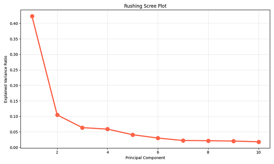

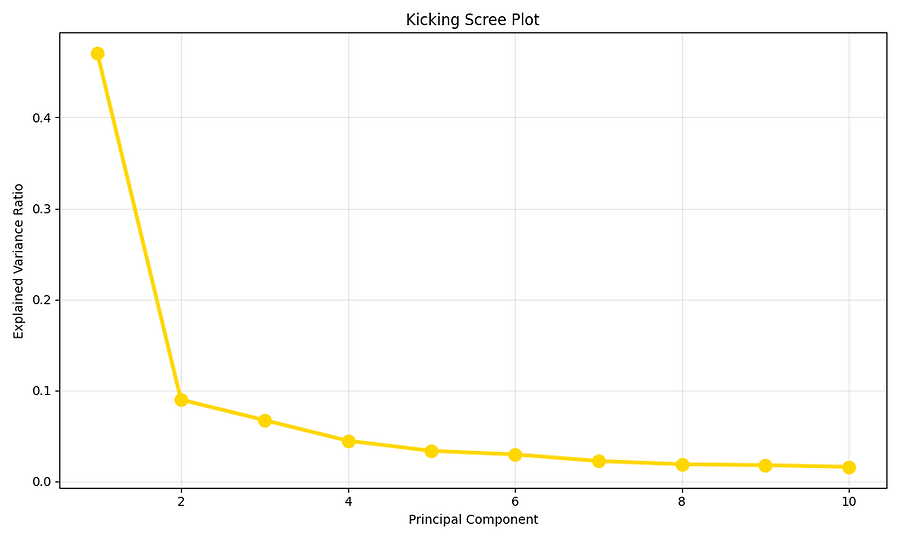

The above graphs are quite fascinating. While each looks fairly similar (almost all scree plots for most data sets look a little something like the above), they tell us that many of the vast collection of columns of data in the original PCA final U-matrix are contributing quite a small amount to the total variance in the data. One only really needs a few of these new principal component eigenvectors to explain most of the variance.
The industry standard at this point in Principal Component Analysis is to let go of all U-columns except those, in decreasing order of significance, that are contributing up to 95% of the variance. So long as we keep those explaining 95% of the variance, the others may be allowed to evaporate away.
The PCA process substantially reduced the dimensionality of the NFL datasets. Depending on position, between 31 and 47 principal components were sufficient to preserve over 95% of the variance originally contained in multiple thousands of features.
It was now time to return to the NFL predictive engine's core purpose and see what would happen when test players were compared to this new, simplified, less-noisy data. Where previously, for the Clustering processes, the new issue causing trouble was the -1 padding elements within the data cube, this PCA process might result in a new source of calamity. The careers of all players were stretched to 100 years, while their career lengths were saved and multipled by 5. The new difficulty is that the test players's career lengths are completely unknown. That's a large portion of the whole basis of this project! The only way to properly compare a test player's info to the new stretch 100 year careers is to allow for the hypothetical possibility that the test player might play for any length of time, from the original given number of years all the way up to possibly 25 years. Each of these options would cause a different amount of stretching (to properly compare to the 100 year stretch data in the PCA datacube), and so each of those different stretch factors must be tested.
By comparing each test player, and to each possible degree of stretching, to each player in the PCA datacube, the predictive machine can once again gather the 30 closest players. It will once again use those 30 closest players to generate a prediction for the median retirement estimate and for the median percentile scores for the rest of that player's career.
Much programming later....
Much much programming later, no final working version of the new PCA-based version of the predictive machine was ever finally made to work. Trying to take the test player, stretch the given years of their career to all possible lengths from immediate retirement to a proposed 25 year long career, compare to the PCA-transformed data, and gather the 30 closest players... proved to simply be too complex a coding challenge to complete within the given time frame of this project.
It is, however, highly worth noting that early test runs did manage to succeed in completing that pipeline from start to finish, but across all three that succeeded, the average retirement error was still 3.1 years, proving that even this quite-complex machine was most definitely not an improvement upon the original method.
The PCA-based predictive machine was a bold endeavour, but ultimately (and for an entirely new reason!) proved to still not be able to handle the core issue so far encountered of how to apply these various machine learning techniques upon data cubes of variable lengthed NFL player careers. For the sake of future research as the project continues, this issue will hereby be coined — "The Jagged Cube Problem".

Conclusions
Principal Component Analysis proved to be an effective method for reducing the dimensionality of the NFL datasets while retaining most of the underlying information. The original data cubes contained serveral thousand features after career stretch and flattening. PCA was able to compress this information into only a few tens of principal components while still preserving over 95% of the original variance. This demonstrates that much of the information contained within the original datasets is highly correlated and could be represented in a much smaller space.
One of the most interesting observations was that players with similar career profiles tended to remain near one another even after the PCA transformations! For example, backup and short-career wide receivers clustered together, while elite long-careered players, like Jerry Rice, clustered together with other historically successful receivers. This suggest that the PCA technique does not only reduce dimensionality in a purely mathematical sense, but actually captures meaningful patterns in player performance.
Overall, the portion of the project demonstrated that PCA can dramatically simplify complex sports datasets while preserving meaningful relationships between alike players. The results suggest that dimensionality reduction can serve as a useful preprocessing step for sports analytics and predictive modeling, although for now practical challenges remain when applying PCA to variable-length career trajectories. New solutions may have to be innovated in chapters to come to better address The Jagged Cube Problem. That... or perhaps there are machine learning techniques best suited for working with data of variable vector length. That will be a fascinating new area of inquisitive investigation as this project proceeds forward.