Decision Trees
Predicting the Predictions,
Teaching the model to self-correct


Overview
Decision Trees are a supervised machine learning technique used for both classification and regression problems. Unlike many statistical models that rely on complex mathematical equations, decision trees make predictions by repeatedly asking a series of simple questions about the input data. The overall structure forms a kind of tree. Each question sends the algorithm down one of two possible paths, depending on the input data. After each question, the data is divided into smaller, more-similar groups until a final prediction grouping can be made.
One of the great strengths of decision trees is their user-friendly interpretability to human eyes. Because each prediction follows a sequence of easily understood decisions, it is possible to retroactively manually trace exactly how the algorithm arrived at a particular result! This ability is both useful for analysis... and fun for observation.
For the sake of this project, decision trees are going to be used to try and "predict the predicions". Most of the machine learning tools so far the project has taken and used the tool directly to try and produce a career prediction for each given NFL player. This time, a full comprehensive survey will be done on the current best predictive model, the K-Nearest Neighbors version armed with median, to see how well its predictions fair with each and every possible test case. Subjects for post-prediction analysis will be things like: Which players does the predictive model predict to retire too early? Which players does it get retirement prediction correct for? Furthermore, within its predictions for future career percentile scores, which players does it predict to play more poorly than they actually performed? For which does it get their performance correct? Players will be 'binned' into various categories based on how well or poorly the machine was able to predict the future of their careers.
This "predicting the predictions" will let the NFL project enter a new phase where, for a given player, a first prediction can be produced, then that same player analyzed by a decision tree to predict how good or bad that prediction is, then based on that the original prediction can be altered / nudged in hopefully a better direction to perhaps give a new and improved better prediction! This is a very exciting new objective for the project, and it with held breath that the research continues on into this chapter.
But first, it would be wise to discuss what decision trees are and how they work. For a proper demonstration, a few specific QBs were somewhat randomly selected, along with an associated given number of years from their careers to be offered to the machine as test data. The usual 30-nearest neighbors version of the predictive engine was run on each their careers and a prediction was generated for how soon they'll retire. Some it predicted to retire too early, some it got correct, and others it predicted to retire too late:
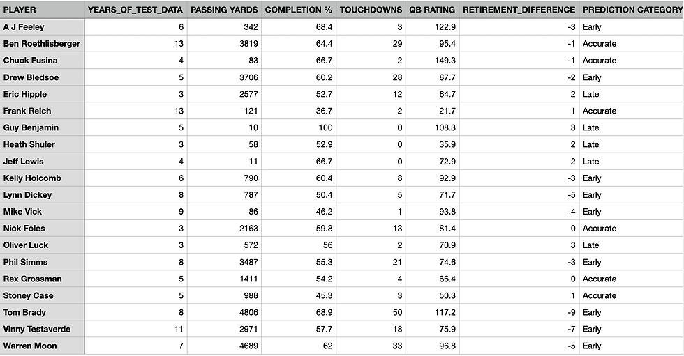
With the simplified NFL dataset above, the objective is to eventually be able to take a new player's data and figure out how their prediction should be classified — early, accurate, or late. For this... enter decision trees. The first thing that must be done is to determine which player statistic should be used as the first decision in the tree. Should the algorithm first split on Years of Test Data? Passing Yards? Completion Percentage? Touchdowns? Decision trees answer this question mathematically by measuring how "good" each possible split is. Two common measure of goodness are Gini Impurity and Entropy. In this demonstration, Gini will be used.
Gini Impurity is a mathematical measure of how mixed the prediction categories are within a group of data. A group in which every player belongs to the same prediction category has a Gini Impurity of 0, indicating a perfectly pure node. Conversely, a group containing a mixture of multiple categories has a higher Gini Impurity. The highest possible Gini Impurity is 1 - 1/k, where k is the number of categories. So in the above example, the max Gini Impurity would be 2/3. The objective of a decision tree is to repeatedly divide the data into groups with a progressively lower Gini Impurity until the players within each group belong entirely (or at least predominantly) to the same prediction category.
For a dataset containing k prediction categories, the Gini Impurity is calculated using the following formula:
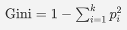
where the pi's represent the proportion of observations belonging to the ith prediction category. Let's do a small demonstration of how this process works.
The first step to do is to calculate the Gini Impurity of the entire dataset before any splitting occurs. This value will serve as the baseline against which every possible split is compared.

The next step is to try out many many different possible places to do the first split. Each column is tested, and within each column, splitting between every pair of neighboring values is tested. Let's give an example.
Suppose one chooses to split the above data based on the column Passing Yards. Suppose the adjacent pair of values, within that column, that are selected is 988 yards by Stoney Case and 1411 yards by Rex Grossman. One defines the split value as being the mean of those two numbers, aka split on 1199.5 yards. The divide results in the following split:


The two new Gini Impurities are calculated:
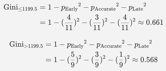
And finally those two new values are averaged together, but only after being assigned weight-values based on how many players were in each group.
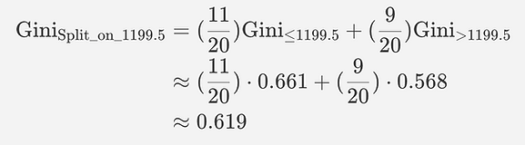
This process is performed upon each column and, within that, upon each neighboring pair of values with the goal of discovering which has the least Gini Impurity:
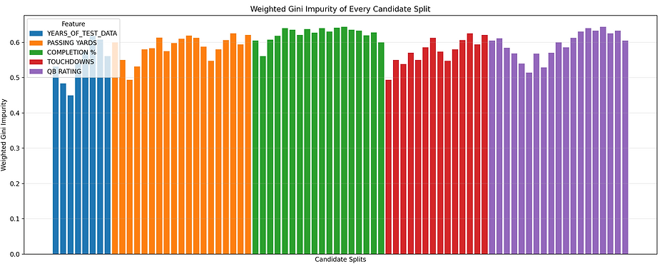
The split is found to be most-optimal when dividing on Years Of Test Data ≤ 5.5, which gives a Gini Impurity values of 0.45. Decision tree formation is a greedy algorithm, so this most-optimal value is selected, and the algorithm never looks back.
In recursive fashion, more splits are then considered, and then more after that. One could, in theory, perform more and more splits all the way down until all the leaf nodes necessarily have values only of one category, but for the decision tree to have legitimacy, usefulness, and readability, often a desired depth is selected before the algorithm is begun. With such a smal demo dataset, perhaps a decision tree of three layers would be wise here.
The full algorithm is run, and this is the decision tree that results:
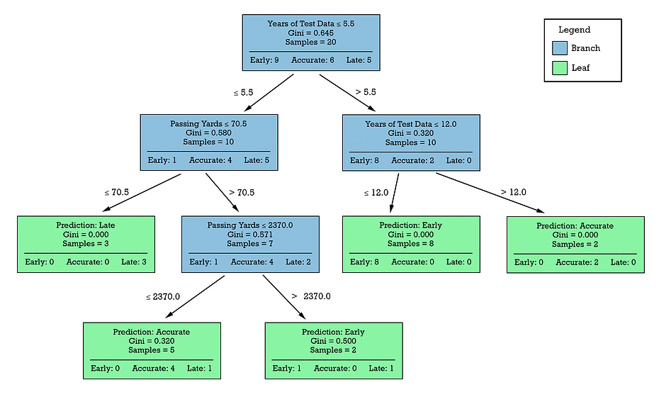
With each branching fork in the path, one can discuss the Information Gain that has occurred there. Information Gain is a quantitative measure of the reduction in Gini Impurity achieved by partitioning a dataset according to that particular feature and threshold. It compares the impurity of the parent node to the weighted average of the impurity of the children nodes produced by the split. Formally, it is defined as:

In a sense, the Information Gain is a way of measure the before and after of performing that particular split. A larger Information Gain indicates that the split produces more homogeneous children nodes and is therefore considered a better partition of the data.
It is important to note that with a large-sized dataset, the full number of possible trees that one could select from is nearly infinite. The total number of just the first split is the number of columns times the number of unique values in that column. The total possible number of different decision trees one could explodes exponentially very quickly, rather like the near-infinite number of possible chess positions. This is why the decision trees are treated as a greedy algorithm, optimizing Information Gain at each step, in order to get a tree that's "pretty good", rather than seeking the theoretical optimal tree, among the nearly infinite possibilities.
That being said... with the full demo tree now complete and visible. Let's do an example test run to see how it is used for prediction. Suppose we take the Hall of Famer Peyton Manning after his 8th season and run him through the decision tree. The year was 2005, and these were his stats that season:

Will the predictive engine predict his career to end too soon, too late? Maybe right on time? Let's find out!
Peyton Manning is entered at the top of the decision tree at the root. The first question is: Is the decision tree being presented with ≤ 5.5 years of test data? The answer is no, so he moves along the right branch of the split. The second question is: Is the decision tree being presented with ≤ 12 years of test data? The answer is yes, so he moves along the left branch of the split. With that, a leaf node is reached, and a prediction is made. That leaf predicts that his classification will be one of 'early'. Let's now examine the original result from the earlier predictive engine and see how he was, in fact, classified in truth.

The decision tree was able, in this case, to correctly "predict the prediction". This is an encouraging sign. As the project enters the next phase and performs real-world use of decision trees, upon much more complex and higher-dimensional data, the goal will yet again be to "predict the predictions". At the end, the predictive engine will be able to spit out its original predictions as before, then examine the associated decision tree for that player, and finally alter its predictions with a suitable 'nudge' to push the predictions (hopefully) in the correct direction. This is an exciting area of research, and it will yet be seen whether or not this concept is efficacious.
Data Prep
The first and largest job that needed to be completed in order to implement a new Decision Tree-based version of the model, one that could perform the "predict the predictions" adjustments, was to manually go through each and every NFL player paired with each and every valid number of years of submitted training data (3 through 10 years) and compute the current version of the machine's 30-nearest neighbors predictive analysis. This code was not hard to compose, but had quite-significant runtime. That code, and the results thereof, are found here:
There were a few important decisions that went into this code. The first was that it's much nicer to give a decision tree a small, tangible number of various columns to choose from. It gives the research meaning. This means that allowing for every individual statistic across every player's entire career, individually per-year, seemed a little out of line with the spirit of what decision trees try and do.
The decision was made to take each player/num_years pair and compute the average of each of the previous three years' worth of data and combine those into a single statistic. This means that for each player, the decision of how much to alter their retirement prediction would be based on their recent performance. Perhaps this would reduce something in the effectiveness of this corner of the project, as it might have been nice to have the decision trees make their choices based on the full, complete player-career knowledge, but it was also important to allow the decision trees to do their work.
Sticking just to, for the moment, the topic of nudging the retirement estimates in a good direction by "predicting the predictions", it became relevant to have a sense of how much the retirements should be altered by. The key question was what should the various bins be to which the players would be categorized. Above, in the demonstration earlier, "early" was defined as ≤ -2, "accurate" was defined as -1 ≤ player ≤ 1, and "late" was defined as ≥ 2. Would these be the best choices? Maybe something else? It wasn't even clear how many bins the players should be divided into!
To assist with these types of decisions, exploratory research was done on the datasets to see how many player predictions had which number of years of retirement errors. To show two examples, here are the bar charts of those values for quarterbacks and for defensive players:


It was eventually decided to group the retirement errors into five classes: ≤ -4, -3/-2, -1/0, 1/2, and ≥ 3. These buckets were chosen to balance the model's simplicity, functionality, and predictive usefulness. It seemed more relevant at this stage in the research to attempt to be humble and aim to "beat placebo", rather than fine-tunededly aim to fully, precisely predict the predictions down to a single year. This philosophy was aimed at making sure to avoid the class main drawback of decision trees, that of overfitting to the data.
Those specific bucket-values were chosen for a variety of reasons. The first was to capture as much of the body of the skewed bell curves above as possible using only small adjustments. This would make sure that the model would not be overcorrecting. Bins of size two seemed reasonable, again to try and dodge the phenomenon of overfitting. In particular, however, this led to the question of whether "accurate" should be as wide as a three year margin, like in the original demo earlier. This seemed to be a little too wide a margin, as it would capture most players and then not adjust their retirement values. It became the objective to have "accurate" be a bin with a width of two years.
With that in mind, the choice became to have it be 0/1 or -1/0. Examining this in a different way, this is similar to asking whether the previous version of the predictive engine was erring "on average" a little towards predicting players to retire too soon or too late. For this, it seemed wise to examine the various mean retirement errors for each player position:
Quarterbacks: −1.245
Rushing: −1.128
Receiving: −1.031
Defense: −1.216
Kicking: −0.794
Visible within these numbers is a slight trend. The previous predictive engine had a tendency to predict players retiring slightly too early. Because of this systematic bias, a retirement error of −1 was classed, then, as a relatively typical outcome and was grouped together with perfect predictions (off by 0 years). This, and a desire to have the central bins be of width two, led to the five classes: ≤ -4, -3/-2, -1/0, 1/2, and ≥ 3.
Next up came the choice of how to address the percentile errors. These are much more complex. Where the retirement error is a singular integer value, the percentile error has unique float value for each year of the rest of that player's career. One immediately obvious way to address this would have been to have a whole nother decision tree for each successive year. This would have, at best, led to dramatic overfitting no matter how well performed. This seemed like a terrible option.
A little bit of exploratory data analysis seemed to indicate that for the average player that the predictive engine was predicting to play too poorly, it seemed to lean on the 'too poorly' side for their entire career. Most players it was universally predicting all of their future seasons either too well or too poorly. With this in mind, it seemed a very reasonable way to go about the project would be to attempt to "predict the predictions" as one float value representing the mean difference between the engine's predictions and the true value of the rest of that player's career across all of the remaining seasons they played. This would be one blanketed nudge applied, as a float value, across all of the years of their prediction. Again, the goal was to beat placebo (making the decision trees useful), while avoiding overfitting.
Towards this end, it became important to get a sense of how much the player predictions were off by, on average, across the various player careers. Here is a glimpse at a summary of those values:

Many different way to bin the percentile errors were considered. My first very simple approach, before seeing the above data, was for the three bins to be ≤ -0.1, -0.1 to 0.1, > 0.1. But upon seeing this info, that seemed to be too severe an alteration.
After much consideration, and a little soul-searching, it was decided to stay humble and make only small changes to the predictions. This would let the decisions-tree-based version of the predictive engine still be primarily based on other less-prone-to-overfitting machine learning tools. The inherent danger was that if one built a heavily, heavily decision-trees based machine, it would be possible to use such small granularity that the predictions would always be 100% accurate. This is because the training data and the test data are the same set! The ultimate real test of this machine is going to be when it is used to predict the careers of current players, for whom the rest of their careers are unknown quantities. In the years to come, that's when this machine will really be able to prove is mettle. A heavy decision tree overfitting machine would not help with this at all.
In the interest of making this portion of the project give only gentle nudges, the ultimate bins decided on were ≤ -0.05, -0.05 to 0.05, > 0.05. If a player's career was determined to be in the ≤ -0.05 category, a nudge not of 0.05 but of 0.07 would be given. This would push a very small number of players too far up, passing 0, but would let most players in that bin get closer to 0. These values could be tweaked and worked with almost ad infinitum. There is much room here left for further experimentation and future refinements.
Code
All of the code used in this portion of the project can be found via the following link. Each small specific experiment run will have a provided link to its own small sub-folder. But here is the link to the larger outer folder that contain all the code:
Results
With all the set-up complete, the data fully prepared, all the choices made, it was finally time to train the decision trees. Ultimately there would be 10 trees, two for each player position — a retirement one and a percentiles one. Below only the full output for quarterbacks will be shown. A separate link will be offered at the bottom with all the other trees.
QB Retirement Decision Tree

QB Percentile Decision Tree
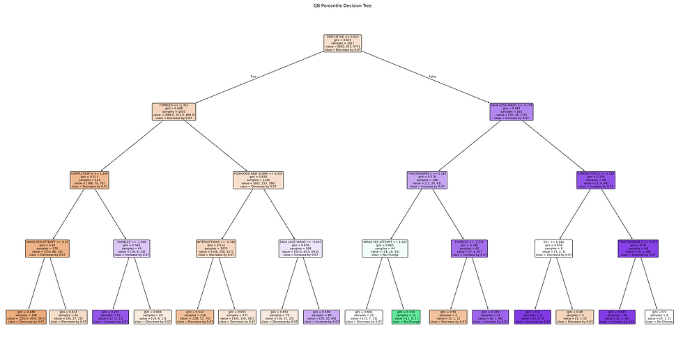
In examining the 10 different complete decision trees, several interesting patterns come into view. Perhaps the most striking is that the Kicking trees are the only ones that are not of uniform depth, with several branches terminating early. This may suggest that kicking performance is easier to classify using a relatively small, simpler structure. It's also possible that this is a direct result of there being less kickers in the database. The root cause is unclear. Another interesting pattern is that across all five retirement trees, Years Revealed consistently appears as the most influential feature near the root of the tree.While this is an intuitive result — players who have already played for long careers and naturally closer to retirement — it provides quantitative confirmation that career length is the dominant factor when refining retirement predictions.
The percentile-adjustment trees also reveal several intriguiging position-specific patterns. One particularly interesting finding appears in the defensive model, where where very best-ranked players who have additionally sustained very long careers universally received the same positive adjustment (with Gini = 0), indicating that original nearest-neighbor predictor systematically underestimates these long-lived defensive standouts. It's time to boost their scores in the predictions. Charles Woodson would be proud! Likewise, the kicking percentile tree contains a pure (Gini = 0) rule showing that for already known weaker kickers, all it takes is their extra-point accuracy to be a little worse, and their whole future careers need to be universally adjusted for the worse. It's fascinating seeing the effect something as small as missing an extra point might indicate about the entire rest of such a player's career!
Beyond these examples, each position develops its own unique collection of influencial features — quarterback percentile being influenced heavily by fumbles, runningbacks's being decided based on the composite HowGood Raw Score. Examining the full, complete decision trees makes for a very interesting read and illustrates that although the overall methodology is consistent across positions, each position group possesses its own distinct statistical signatures that govern how positions should be refined.
Predicting the Predictions
With the decision trees all complete, it was finally time to build the decision tree-based version of the predictive engine. The previous "high score" version of the machine would be run, using 30-nearest neighbors armed with median, to generate an initial prediction. Then after that prediction is fun, that player's most recent 3 years of statistics would be averaged to prepare the player's info for entry into their position's two associated decision trees. That player would then be classified by the decision trees into the appropriate binning for how to nudge their career prediction. And then finally a new prediction would be generated!
There was, however, a few important decisions yet to be made. Suppose a player's current career prediction is 4 seasons, and the retirement nudge, suggested by the decision tree, is to trim it down by 2 years. Which seasons should be trimmed off? There are many different ways to possibly do this, but it seemed wisest to leave the later years intact. This is because most players tend to play significantly worse in their final season or two, and that "career fall off" is being predicted within the 30-closest players analysis. Were the project to simply delete values from the end of the vector, it seems less than valid to simply pretend that the new nudged player's shorter career will magically not have that fall off at the end. Deleting from the start of the prediction seemed like the best way to proceed.
Next, how does one add to the career vector if more seasons are to be predicted? It seemed wisest to keep the general shape and structure of the career and simply stretch it out to be longer. Again, there were many possibilities, but this one was selected. Suppose the current career is of the form [A,B,C]. And suppose that career needs to be lengthened to be 7 years instead. Instead of either [A, A, A, A, A, B, C], possibly artificially inflating how well they played over their career, or [A, B, C, C, C, C, C], likely significantly undervaluing how well they'll play for most of their career, the choice was made to stretch the career out to instead look like [A, A, A, B, B, C, C]. This is one of many decisions in this portion of the project that could be further-tested and refined for possible performance improvements
Lastly, and most difficult, what should the engine do when the original prediction was for immediate retirement, and yet the new 'nudged prediction' asks for an addition two years? It was chosen in this case to simply duplicate that player's last year of performance.
With that, all decision had been mad, the decision trees were complete, and all was ready to go. The final test experiment with 10000 players, and the same random seed as usual, 333, was performed. This is the result:
Before Decision Trees

After Decision Trees

Retirement Adjustment Distribution:
-3 Years —— 2.13 %
-1 Year —— 10.68%
+1 Year —— 83.85%
+ 3 Years —— 0.71%
+ 4 Years —— 0.63%
Percentile Adjustment Distribution:
-0.07 —— 31.97%
+0 —— 45.28%
+0.07 —— 20.75%
Retirement Nudges:
Improved —— 43.52%
Worsened —— 56.40%
Percentile Nudges:
Improved —— 48.09%
Worsened —— 51.91%
These results are fascinating. For all that careful decision tree work, it actually made the predictive engine perform worse! This was quite a startling and unexpected result. After much consideration, a few theories arose for why this might have come to pass:
1.) It's possible the corrections were too coarse. This is the most optimistic explanation, as it imagines that properly performing decision trees would help, but these decision trees did not. It's possible that small, gentle nudges might have assisted, and perhaps these were too abrupt. For all of the attempts to scale down the power of the corrective pushes that went into construction of this machine, perhaps it was still too much of a good thing.
2.) It's possible the 30-nearest neighbors machine was already close to optimal. While this seems a little far-fetched, it's possible that attempts to improve upon that version of the machine with decision trees would never have worked. It's possible that the nearest neighbors already encode many subtle relationships between career trajectory and player statistics, and there may have been relatively little remaining error for the decision trees to correct. Instead of discovering new information, the tree may have often introduced unnecessary adjustments to predictions that were already reasonably accurate.
3.) It's possible (perhaps even likely!) that the nearest-neighbor errors may not be predictable. This, if true, would be a fascinating scientific conclusion. This would hint that the entire philosophy of attempts to use decision trees here may be flawed. For decision trees to assist the predictions, an underlying axiom must be taken of "the errors made by nearest neighbors follow predictable patterns." Perhaps they don't. Perhaps those remaining errors, both large and small, are primarily random variations due to injuries, coaching decisions, changes-of-team, pure luck, or countless other factors that simply aren't captured by the datacubes. If this is true, then no decision tree work could consistently improve the model.
That being said, in an attempt to not give up too soon, one last push was made to see if decision trees could be used in any context to assist the predictive engine. Analysis was done upon a large body of players, with a new random seed for scientific legitimacy, to see if perhaps the decision trees were helpful, but only for certain classes of players. Players were separated by their player-position and by the number of years of given data, with the following results.

Here, finally, we can see that the decision trees were not all bad. For every single position and stage of career, they managed to improve at least one of retirement or percentile... while often worsening the other. It was decided to reject and "turn off" the decision tree nudges for all of these categories of players except those for which it was beneficial for their predictions on both retirement and percentile scores as well. Recall, one more time, that the above study was done with a unique new random seed, to try and prevent overfitting. A new, final, and last rendition of the decision trees version of the predictive engine was scripted to run in the following manner:
Perform the traditional 30-nearest neighbors analysis, armed with median (the current high score holder) and alter only those players who are either quarterbacks early in their career or running backs late in their career. This would seemingly use a very moderate, humble amount of decision tree nudging, only where it was shown to be most efficacious. The code was written, the experiment performed, and these were the final results:
Decision Trees (reduced usage)
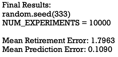
This final, more humble version of using decision trees to nudge the predictions finally paid off and gave slightly, slightly better results than the original. While it was still perhaps a disappointing result, considering the initial excitement entering this phase of the project, it none the less was the new high score. Even so, there is some argument to be had as to whether or not the selections of exactly which player positions to apply the decision trees to had a small amount of overfitting as part of the analysis. Is it "fair" to use decision trees only for young quarterbacks and aging running backs? This choice was made only after knowing that those were the two groups for whom the decision trees happened to perform well. While the result is still a new and exciting best version of the machine, perhaps one would be wise to tread lightly upon decision tree-based analytic predictive models.
Conclusions
Despite the relatively modest improvement ultimately achieved by the decision trees, this phase of the project was far from unsuccessful. One of the primary goals of any machine learning investigation is not simply to discover what works, but also to discover what does not. The experiments performed here demonstrated that decision trees are indeed capable of learning meaningful patterns from historical NFL data, but that those patterns do not necessarily consistently translate into better predictive performance when applied broadly.
Ultimately, the strongest version of the predictive engine remained rooted in the comparatively simple nearest-neighbors approach, enhanced only by a very conservative and carefully selected use of decision tree corrections. While the final gains were small, they nonetheless represented a new best-performing version of the machine!
It is possible that with further work, and more nuanced refinements, decision trees could play some role in a breakthrough that would really decipher the patterns of predicting when the predictive engine will do well and when it will do poorly. The trouble here is that when applied too broadly (trying to nudge most players' career predictions), the method backfired and gave worse than placebo results. That being said, there still might be wonderful room to work on researching analyzing the predictions and trying to learn the science of when the machine works well and when it fails to.
Ultimately, the core problem with this method is that given only three years of the early part of an NFL player's career, it really is very hard to tell whether you're looking at a young Tom Brady or a young Carson Wentz. There is very real and very deep ambiguity in trying to predict the future of an NFL player's career. Consider the Denver Broncos's massive trade to acquire Russell Wilson in the hope of rekindling the fire of his early superbowl years. It's an incredibly hard job trying to predict how well a player will do in later years, based on previous years. And as difficult as that is, trying to then recursively predict the accuracy of the machine learning predictions themselves, might ultimately be a bit too much.