Clustering
Before being able to start working on adding Clustering techniques to the project, an earlier prerequisite step that needed to be completed was taking the previous complete version of the NFL data mining predictive machine and coming up with a way to quantitatively, numerically evaluating it with a score indicating how close its predictions are to reality. This extra bonus page explains that full process:
The above work led to the first ability to quantitatively analyze the accuracy of the model's predictions and assign the accuracy a numerical score. The current "high score", if you will, is:

This is the score that the project will now attempt to best by using more and more elaborate and advanced machine learning techniques as the project continues. For now, the next step is to try out adding Clustering to the project.
Overview
K-Means Clustering is an unsupervised learning technique that partitions a data set of n points into k clusters, grouping together points that are similar according to a chosen distance metric. The algorithm assignms each point to the cluster whose centroid is nearest, thus forming clusters of closesly related observations.
Hierarchical Clustering, a related but slightly different technique, forms a tree-line structure called a dendrogram. Each data point begins as its own cluster, and the algorithm repeatedly merges the most similar clusters, recursively.
Visual examples of those two processes can be seen here:
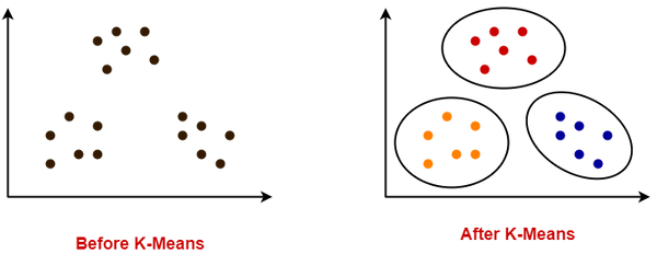
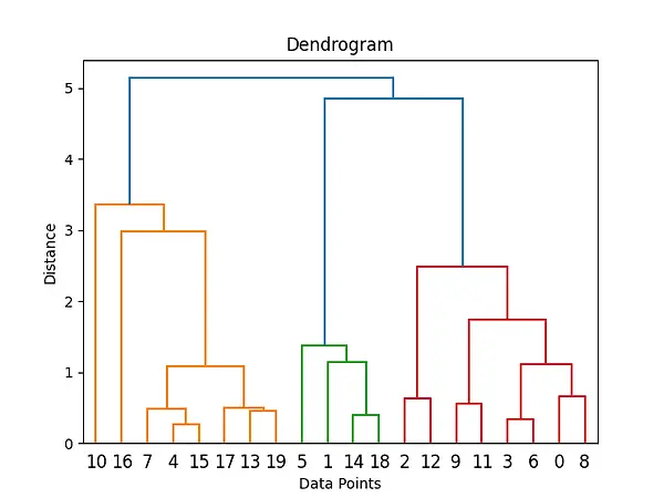
This project will employ K-Means Clustering, armed with Euclidean distance, to measure the similarty between player career vectors. It's important to note that K-Means Algorithm requires vectors of uniform length, so players with shorter careers will have to have later seasons added to their careers, with dummy stand-in statistics, in order to be able to run K-Means.
Later Hierarchical Clustering will be tested, using cosine similarity instead of the Euclidean measure, to generate a dendrogram tree diagram of more-similar players clumped together onto closer branches.
Both K-Means and Hierarchical styles of clustering are very well-studied, well-trusted methods for grouping similar data points together. It is with much excitement that the project ventures into these waters with the hopes of finding that one or the other machine learning technique will drive the retirement error and or the predictive error even lower. These discoveres may provide additional insight into career development and retirement trends among NFL players.
Data Prep
K-Means Clustering requires unlabeled numerical data. Categorical data would not be applicable here. Neither of these presents much of an issue with this project, as the NFL data is all numerical in form already. This means that the same five data cubes used throughout the project — QBDataCube.csv, RushingDataCube.csv, ReceivingDataCube.csv, KickingDataCube.csv, and DefenseDataCube.csv — can all have K-Means Clustering implemented upon them with no changes required. For a small example of what these data cubes look like, here is a glimpse inside the kicking data cube:

A few important details are worthy of note. Each "node" that the project will cluster represents a player's entire career. In the above diagram, without any further processing, it would be impossible to run the clustering algorithm on both Aaron Elling's career (who played for 3 seasons) and Adam Vinatieri's career (who played for 24 seasons). Pre-processing must be performed to make all the vectors be the same length.
To do this, within each data cube, the player with the longest career length is sought out. In the case of NFL kickers that player is Morten Anderson who played for 26 years from 1982 through 2007, mostly on the New Orleans Saints and the Atlanta Falcons. All other players's careers are then "padded" with some sort of dummy variable. The number -1 was chosen. While this is standard practice for performing K-Means Clustering on vectors of variable lengths, it does put significant weight upon that newly generated number -1. This means that the clustering will be heavily influenced by how long players's careers were, with players of similar career lengths being much more likely to be clumped together. Whether that serves the predictive engine well or poorly will yet be seen.
A link to the preprocessed data is found here:
Code
All of the code used in this portion of the project can be found via the following links. Each small specific experiment run will have a provided link to its own small sub-folder. But here are the links to the larger outer folders that contain all the code:
Results
K-Means Clustering
K-Means Clustering was incorportated into the project in the following fashion. First, the five data cubes, containing all the players in NFL history, were gathered, and then players of shorter careers had their careers "padded" to be of equal length with the longest career in the data set. The padding number chosen was -1, to influence the clustering to focus more on grouping together players of similar career lengths. For a distance metric, the standard Euclidean distance-between-vectors measure was used. This method resulted, separately for each type of player being studied — QB, running back, kicker, etc — in the predictive engine grouping together like players into K distinct clusters. An initial value of K=50 was chosen. Other values of K will be carefully investigated later.
To give a sense of what those clustered looked like, below is a link to a similar style of clustering, but with K=25 clusters instead. The K=25 clusters better demonstrate how the machine is clumping the players together than K=50, which has tiny little clusters and is harder to interpret by eye.
Using the value K=50, the predictive engine was set to run with its new K-Means Clustering-based style of predicting. This was the result:
K-Means Clustering

This result was quite surprising, as it was dramatically much worse than the previous version of the machine. Most notably the mean retirement error of 3.2960 was a whopping 1.4645 years further off, on average, than the previous version! Where last time the results were incrementally improving at the magnitude of 0.0005 or so, this massive leap up is a sign that perhaps this version of the machine simply fundamentally doesn't work.
That being said, a full battery of tests were performed across a variety of values of K to see if any might have better predictive abilities. Perhaps the poor results were simply due to the choice of K. This is the result of that experiment:
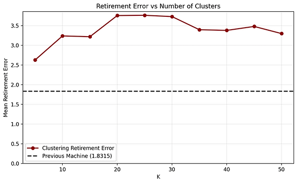
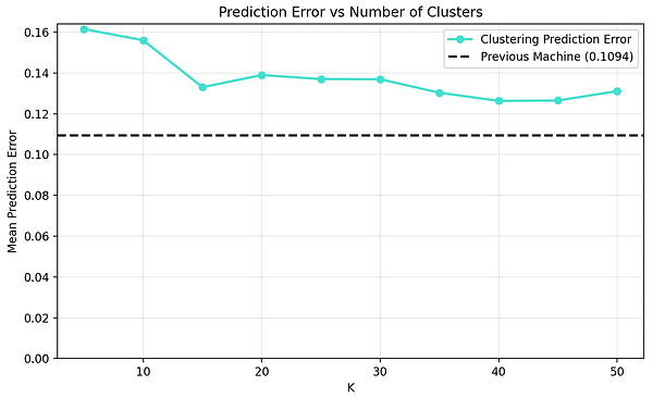
As seen above, all various values of K had both the shockingly worse predictive abilities for retirement, as well as the much more moderately worse predictive abilities for the actual career strength of the tested players. The level to which K-Means algorithm failed at this was startling.
In the interest of rigor and complete analysis, there was at least one slightly more advanced technique that should be employed to determine best values of K, before moving on.
In searching for the optimal value of K, it is often wise to use a Silhouette plot. The Silhouette Method is a technique for finding the best value of K. It measures how similar points are to other points in their own cluster vs other clusters. Higher values indicate better separation between the clusters. Here, as an example, is the Silhouette plot for QBs.

The optimal values of K, using the Silhouette Method, turned out to be:
QBs —— K=18
Runningbacks —— K=12
Wide Receivers —— K=13
Kickers —— K=24
Defense —— K=20
Using these numbers for K, for each class of NFL players,
the machine was redesigned. This was the result:

This, very interestingly, performed worse on both retirement prediction and career prediction than even the earlier, simply K=50 version! As for what may be the mathematics behind the worse predictions, even with the more perfected clusters, the author of this cannot even hesistate a guess! Quite a surprising, unexpected result.
At the end of all this experimentation, it seems that K-Means Clustering might simply be the wrong technique for this project. It does not seem to be assisting in predicting NFL players's future careers.
Hierarchical Clustering
With the results of K-Means Clustering being so unhelpful, the Hierarchical Clustering portion of the project was entered with great skepicism. None the less, it it is important to be thorough, and so a full examination of Hierarchical Clustering was in order next. The Hierarchical Clustering was set up to once again use the "padded" career stats, with players with shorter careers given a -1 for all stats in all future seasons to match the players with the longest careers.
Hierachical Clustering builds its clusters in a recursive fashion. It begins by assigning each player being their very own cluster. Then with each loop, it clumps together the two most-similar clusters into one larger cluster. Viewed as a progression over time, this creates a kind of a tree structure called, in this specific context, a dendrogram. The dendrogram, on the horizontal axis, shows which players are clustered together, and, on the vertical axis, how relatively far apart their careers are.
A worthy fact to note is that Hierarchical Clustering is often performed by comparing vectors using Cosine Similarity, and not the Euclidean vector distance measure. Cosine Similarity takes the two vectors and computes their dot product, divided by their two vector magnitudes. This choice of measurement allows the Hierarchical Clustering to focus more on the comparative 'shape' of the vectors, rather than focusing purely on the magnitudes of the elements in each vector.
To give a demonstration of what Hierarchical Clustering looks like, here is the full dendrogram for all NFL quarterbacks in history:
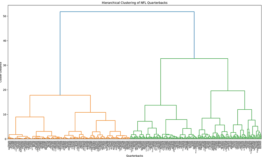
This, while perhaps artistically pleasing, is nearly unreadable! To produce a more useful dendrogram for learning purposes, attention will be reduced to just 40 recent quarterbacks who each had a long career. This will hopefully give us just famous quarterbacks with recognizable, household names:

An immediate thing worthy of note is that we find Tom Brady's career most-closely grouped with those of Brett Favre, Drew Brees, and ... Vinny Testaverde? That's quite odd. One might have expected to find him closely linked with Peyton Manning, as another dominant quarterback of the same era. Mostly likely what this tells is that Hierarchical Clustering is not particularly ideally suited to this NFL research, as it seems to be primarily lumping QBs together based on simply how long their careers were. To test this hypothesis, the code above was ran again, but instead of displaying the players's names, it was programmed to simply have it display their career length:

Indeed, with almost no interference or statistical noise at all, the Hierarchical Clustering is simply lumping together players strictly based on the duration for which they played. The -1 padding elements seem to be dominating the research.
That being said, perhaps there is some wisdom to this way of viewing the historical NFL players. The Hierarchical Clustering seems to be strongly leaning towards focusing almost exclusively on player career length only, at the expensive of all else.
Inspired by this, a new version of the machine was designed. It follows the above model to sort players into small clusters based exclusively on their career lengths. It then takes the test player, compares their career to the centroids of all those clusters, and tries to see where they most closely fit in. Upon being sorted into a cluster, that test player is then given a prediction for the rest of their career based on the statistics of the centroid of that cluster.
While not strictly using Hierarchical Clustering, this version of the machine is "inspired" by the Hierarchical Clustering dendrograms above. This is how its predictions turned out:
Hierarchical Clustering-Inspired

This version of the predictive engine is even more dramatically wrong in its predictions than the K-Means Clustering version. The experiment has been performed, the results are in, and this version of the predictive machine should be abandoned.
Conclusions
The goal of this section was to investigate Clustering techniques, learn about them, and see if they could improve the NFL career predictive engine. Considering how generally useful K-Means Algorithm is, it was quite shocking and unexpected to find how catastrophically it failed to be able to properly predict player careers. Upon first inspection, this author would never have thought that the previous system of finding the 30 closest players, and taking the median of their career percentile scores, would have resulted in such a dramatically better prediction.
What's worthy of note and possible future consideration is that the method of finding the 30 closest players and studying them... is, in a fashion, a somewhat simplistic way to generate a 'custom cluster' for each player. The 30 closest players form a kind of a cluster of sorts, and the median then provides a kind of a centroid for that cluster. With that way of thinking, it's quite a shock that using more conventional clustering techniques performs so much more poorly.